

In this blog post, we will explore the intricate and complex world of stocks. We'll delve into several methods used to accurately predict market trends and movements. As it can be an overwhelming topic, I've simplified the concepts so everyone can quickly grasp them. I hope you find this informative and enjoyable to read.
WHAT IS THE STOCK MARKET?
A stock market is a place where equity shares of companies are bought and sold by the participants (buyers and sellers of stocks).
The participants can be investors and traders who seek profits over the short time or the long run.
The investors mainly have a long-term horizon and benefit from capital appreciation over time.
Traders, however, look for quick profits by focusing on the small price changes in equity shares which mostly last for a few minutes or the whole trading session
PROBABILITY IN THE STOCK MARKET
In the stock market, there are various indicators, represented on a daily chart, utilized to anticipate the next move in the market. These formulas use probability in their calculations to predict trends. Brokerage firms often provide software and online platforms that can provide buy and sell signals directly. It's important to understand these indicators when making investment decisions.
NORMAL RANDOM VARIABLE
·Normal distribution, also known as the Gaussian distribution, is a probability distribution that is symmetric about the mean, showing that data near the mean are more frequent in occurrence than data far from the mean. The width of the curve is defined by the standard deviation
In graphical form, the normal distribution appears as a “bell curve”
The assumption of a normal distribution is applied to assess prices as well as price actions.
Traders may plot price points over time to fit recent price action into a normal distribution.
The further price action moves from the mean, in this case, the greater the likelihood that an asset is being over or undervalued.
Traders can use the standard deviations to suggest potential trades. This type of trading is generally done on very short time frames as larger timescales make it much harder to pick entry and exit points.
Application of the normal random variable in the stock market
Normal distribution, also known as the Gaussian distribution, is a probability distribution that is symmetric about the mean, showing that data near the mean are more frequent in occurrence than data far from the mean. The width of the curve is defined by the standard deviation.In graphical form, the normal distribution appears as a “bell curve”
The assumption of a normal distribution is applied to assess prices as well as price actions. Traders may plot price points over time to fit recent price action into a normal distribution. The further price action moves from the mean, in this case, the greater the likelihood that an asset is being over or undervalued. Traders can use the standard deviations to suggest potential trades. This type of trading is generally done on very short time frames as larger timescales make it much harder to pick entry and exit points

Let’s try to answer a few questions with the curve above
1) What is the probability, for any given day, of a loss greater than 2%?
2) What is the probability, for any given day, of a return between 0% and 1%?
3) What is the probability, for any given day, of a gain or loss of 3%?
1)

2)

We use Q-table to find the final probability Since we cannot directly compute the probability of a Gaussian random variable. P=.6844-(1-0.5239)=0.21

3)

This plot indicates that 10% of the daily returns of apple are eithera loss or a gain of3%. This means that the stock is veryvolatile on a given day.
CONCLUSION Like so many indicators in our statistical indicators, we try to choose the best fit for the occasion, but we don't really know what the weather holds for us. The normal distribution is omnipresent and elegant, and it only requires two parameters (mean and distribution). However, many situations, such as hedge fund returns, credit portfolios, and severe loss events, don't deserve the normal distributions The elegant math underneath may lead you into thinking these distributions reveal a deeper truth, but it is more likely that they are mere human artifacts. For example, all the distributions we reviewed are quite smooth,but some asset returns jump discontinuously.
Prediction of the stock market price is a series of mathematical operations applied on the independent variable. In our case we make use of a few interesting domains like machine learning ,Deep learning which are pure mathematics
Deep learning is a subset of machine learning, which is essentially a neural network with three or more layers.
These neural networks attempt to simulate the behavior of the human brain—albeit far from matching its ability—allowing it to “learn” from large amounts of data.


Neuron:

Parts of Neuron:
Following are the different parts of a neuron:
Dendrites
These are branch-like structures that receive messages from other neurons and allow the transmission of messages to the cell body.
Cell Body
Each neuron has a cell body with a nucleus, Golgi body, endoplasmic reticulum, mitochondria, and other components.
Axon
Axon is a tube-like structure that carries electrical impulses from the cell body to the axon terminals that pass the impulse to another neuron.
Synapse
It is the chemical junction between the terminal of one neuron and the dendrites of another neuron.

Fun fact: There are about 86 billion neurons in our human brain. We try and replicate this functioning in deep learning. Simple Ann:

An Artificial Neural Network in the field of Artificial intelligence where it attempts to mimic the network of neurons that makes up a human brain so that computers will have the option to understand things and make decisions in a human-like manner. The artificial neural network is designed by programming computers to behave simply like interconnected brain cells. There are around 1000 billion neurons in the human brain. Each neuron has an association point somewhere in the range of 1,000 and 100,000. In the human brain, data is stored in such a manner as to be distributed, and we can extract more than one piece of this data when necessary from our memory parallelly. We can say that the human brain is made up of incredibly amazing parallel processors. We can understand the artificial neural network with an example, considering an example of a digital logic gate that takes an input and gives an output. "OR" gate, which takes two inputs. If one or both the inputs are "On," then we get "On" in the output. If both the inputs are "Off," then we get "Off" in the output. Here the output depends upon the input. Our brain does not perform the same task. The outputs to inputs relationship keep changing because of the neurons in our brain, which are "learning."
Input Layer:
As the name suggests, it accepts inputs in several different formats provided by the programmer.
Hidden Layer:
The hidden layer presents in-between input and output layers. It performs all the calculations to find hidden features and patterns.
Output Layer:
The input goes through a series of transformations using the hidden layer, which finally results in output that is conveyed using this layer.
What happens inside an artificial neuron(node)?

Initially, all biases are 0, and weights are given some random value and not zero but some random number.This is because on further differentiating the loss function will be the same for all the weights and they learn the same feature for all the iterations leading to a poorly defined model. Basically not moving down the gradient descent curve.
We first sum up inputs with the product of their respective weights and then add bias, if any.Then activation function is applied on the (∑wi*y(i-1) +bi) where,
Wi is the weight in the node in ith hidden layer;
Y(i-1) is the output from the node in the previously hidden layer;
Bi is the bias ;
But using a neural net like mentioned above is impractical for stock market prediction because we don’t take care of the present input(todays stocks statistics) which affects our prediction. Hence we use a Recurrent neural network.It is similar to a simple ann but has feedback

Here Xt-1, Xt,Xt-1 are inputs at time t-1,t,t+1 and so on...
There are many activation functions:

Output at ith layer=f(∑(wi*yprev) +bi). This process repeats till the output layer is reached, and some output is predicted. This process is called feed-forward propagation. Now this predicted output needs to be assessed if it is right or wrong.
Let us assume the case :

Assuming we have 1000 combinations, (1000^25) =(10)^75combinations of weight. Worlds' fastest super computer, operates at a speed of 93pflops=93*10^15 floating operations per second. Being generous and assuming each evaluating each combination takes only one floating operation. On dividing it will still need 3.40*10^50 years to come up with the best combinations of the weights. Hence is why we use the cost function and introduce a concept of gradient descent. Most popular cost function is the mean squared error(MSE) which is given by (yexp-y)2/2 (for output) Cost function basically tells us how close our predicted value is with the already existing datas output(or can also be said as the sum of all errors at individual layer.

So basically,Our aim here is to reduce this function as much as possible, Here we introduce a concept called gradient descent,next step that takes place is called backpropagation which is one of the most crucial steps as we update our weights at various stages
GRADIENT DESCENT
What Is a Gradient?
A gradient measures how much the output of a function changes if you change the inputs a little bit. A gradient simply measures the change in all weights with regard to the change in error. You can also think of a gradient as the slope of a function. The higher the gradient, the steeper the slope and the faster a model can learn. But if the slope is zero, the model stops learning. In mathematical terms, a gradient is a partial derivative with respect to its inputs.

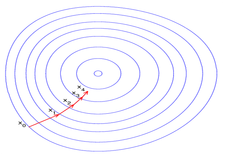
Imagine a blindfolded man who wants to climb to the top of a hill with the fewest steps along the way as possible. He might start climbing the hill by taking really big steps in the steepest direction, which he can do as long as he is not close to the top. As he comes closer to the top, however, his steps will get smaller and smaller to avoid overshooting it. This process can be described mathematically using the gradient. Imagine the image below illustrates our hill from a top-down view and the red arrows are the steps of our climber. Think of a gradient in this context as a vector that contains the direction of the steepest step the blindfolded man can take and also how long that step should be.
We are basically back-propagating the error into the neural net and updating the weights. Given by the following equation. The backpropagation algorithm is based on common linear algebraic operations - things like vector addition, multiplying a vector by a matrix, and so on.
How does Gradient Descent work?
Instead of climbing up a hill, think of gradient descent as hiking down to the bottom of a valley. This is a better analogy because it is a minimization algorithm that minimizes a given function. The equation below describes what the gradient descent algorithm does: b is the next position of our climber, while a represents his current position. The minus sign refers to the minimization part of the gradient descent algorithm. The gamma in the middle is a waiting factor and the gradient term ( Δf(a) ) is simply the direction of the steepest descent.

Applying this analogy in our context,

We are basically back-propagating the error into the neural net and updating the weights. Given by the following equation. The backpropagation algorithm is based on common linear algebraic operations - things like vector addition, multiplying a vector by a matrix, and so on. Equations for the calculation of backpropagation:

These could seem a little overwhelming at first,but it is simple linear algebra with matrices considering all nodes in a given layer.
Analysing gradient descent:
1) Batch gradient descent: works well for quadratic cost functions. 2) Stochastic gradient descent: Works for almost any cost function with higher accuracy. In a nutshell, this is how a recurrent neural network works. Again, there are two problems with using this architecture. Exploding gradient: When we have a large amount of data in the data set say 50 days closing price for which we will have to use 50 neurons unrolled, on only considering w2.The output is a huge value and this leads to taking huge steps on the cost function.

Vanishing gradient: When we have a large amount of data in the data set say 50 days of the closing price for which we will have to use 50 neurons unrolled, only considering w2.The output is a very small value(negligible). Hence we end up hitting a maximum number of steps before getting the right value.

To overcome this issue, We use LSTM(Long Short Term Memory) which is a special type of Recurrent neural network.LSTM only uses activation functions like Tanh(which maps a value between -1 to 1 ) and sigmoid function (which maps a value from 0 to 1). It has two lines Cell state which represents long term memory,they don’t have any weights directly attached to them. Hence can flow to the output without facing problems like vanishing/exploding gradient and another line represents short-term memory which is directly connected to the weights and can be altered. LSTM Structure:

This is just, ONE node of the neural net. Essentially,it is composed of two lines. One is the Long term memory line(This line is directly connected to the output and each node cannot directly access this line(Ct)). Preventing vanishing and and exploding gradient. The other one is called short-term memory line(this line contains short-term information. These lines (ht) are directly accessed and made changes on ,by the node. Note that we only use sigmoid and tanh functions as activation functions. Since sigmoid function maps a value within range (0,1) and tanh maps a value within a range(-1,1). There are three gates, Forget gate(on the left), Input gate (in the middle),Output gate(on the right). Let us learn them individually.
An LSTMneuron has three gates:
Forget gate:we apply sigmoid function on the accumulated already existing short term memory and input,The output gives the percentage of already existing long-term memory to remember.
Input gate:we multiple the outputs of the sigmoid (tells us how much of potential long term memory needs to be remembered and Tanh function(potential long term memory is created)
Output gate: updates the short time memory by finding potential short term memory using the updated long term memory by applying Tanh on it,and updates the short term memory after recognizing how much percentage of it needs to be remembered.
Below,is the code to implement the Stock prediction model using real-world data.I have attached with this Implementation, the link to get the data set.Let us know,if you want me to explain the code. Until then, Happy learning 😉.
Link for the dataset: https://finance.yahoo.com/quote/MSFT/history/ Working code for stock price prediction:
import pandas as pd
df = pd.read_csv('MSFT.csv')
import datetime
def str_to_datetime(s):
split = s.split('-')
year, month, day = int(split[0]), int(split[1]), int(split[2])
return datetime.datetime(year=year, month=month, day=day)
datetime_object = str_to_datetime('1986-03-19')
df['Date'] = df['Date'].apply(str_to_datetime)
def windowed_df_to_date_X_y(windowed_dataframe):
df_as_np = windowed_dataframe.to_numpy()
dates = df_as_np[:, 0]
middle_matrix = df_as_np[:, 1:-1]
X = middle_matrix.reshape((len(dates), middle_matrix.shape[1], 1))
Y = df_as_np[:, -1]
return dates, X.astype(np.float32), Y.astype(np.float32)
dates, X, y = windowed_df_to_date_X_y(windowed_df)
dates.shape, X.shape, y.shape q_80 = int(len(dates) * .8)
q_90 = int(len(dates) * .9)
dates_train, X_train, y_train = dates[:q_80], X[:q_80], y[:q_80]
dates_val, X_val, y_val = dates[q_80:q_90], X[q_80:q_90], y[q_80:q_90] dates_test, X_test, y_test = dates[q_90:], X[q_90:], y[q_90:]
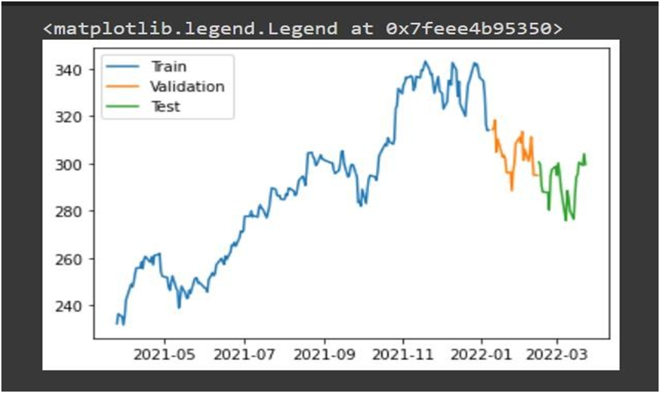
plt.plot(dates_train, y_train) plt.plot(dates_val, y_val) plt.plot(dates_test, y_test)
plt.legend(['Train', 'Validation', 'Test'])
from tensorflow.keras.models import Sequential
from tensorflow.keras.optimizers import Adam
from tensorflow.keras import layers
model = Sequential([layers.Input((3, 1)),
layers.LSTM(64),
layers.Dense(32, activation='relu'), layers.Dense(32, activation='relu'), layers.Dense(1)])
model.compile(loss='mse',optimizer=Adam(learning_rate=0.001), metrics=['mean_absolute_error'])
model.fit(X_train, y_train, validation_data=(X_val, y_val), epochs=100) train_predictions = model.predict(X_train).flatten()
plt.plot(dates_train, train_predictions) plt.plot(dates_train, y_train)
plt.legend(['Training Predictions', 'Training Observations'])

References:
Commenti